Choose a model, enter the data, and make sense of the result. A fit is useful only when you know what its parameters mean.
Original SAT-style teaching examples. Screenshots show actual calculator sessions; the complete steps and results are also written out. No sign-in is needed, and the practice below does not change account progress.
Use Add Item → Table for paired data. Check the headers: these examples use x₁ and y₁. A later table may be named x₂ and y₂; then change the model input to match.
A regression uses ~, not =. In a copied input, the code \sim creates that tilde. x_{1} means x-subscript-1.
For fractions, exponents, square roots and logs, the copy inputs below use explicit Desmos-compatible math notation. Do not copy smart quotation marks or screenshots into an expression.
Use the current parameter variables in later calculations. Avoid retyping rounded displayed coefficients.
Worked problem
Fit a line, then answer the question
A linear model is appropriate for these measurements. Estimate y when x = 3, then find the residual at x = 4.
Why this approach works
The table holds paired measurements. x₁ and y₁ refer to whole columns, while m and b are the two numbers we want Desmos to choose. A line is appropriate here because the problem says to use a linear model; it is not something the calculator establishes just by producing a line.
The tilde asks for a best fit. For each row, the model predicts mx + b; observed minus predicted is its residual. Least squares chooses m and b to make the sum of squared residuals as small as possible. Squaring stops positive and negative errors from canceling and gives larger misses more weight.
Defining f lets us ask the fitted model a new question. f(3) means “what does this model predict at x = 3?” It is not a request for the measured table value. Subtracting f(4) from the observation 27 measures the vertical gap at that same x-value.
Enter these paired values into a new Desmos table.
x₁
y₁
0	12
1	15
2	19
3	22
4	27
Copy the table data
0 12
1 15
2 19
3 22
4 27
Paste into an empty expression to create a table. Or choose Add Item → Table and enter the numbers manually.
What to enter
Choose Add Item → Expression. Paste each input into a separate expression line. Use a fresh calculator for each worked problem, including the model comparison. Every example includes its own table and setup.
y_{1}\sim mx_{1}+b
f(x)=mx+b
f(3)
27-f(4)
Do this step by step
Put the x-values in the first table column and the matching y-values in the second. Keep each pair on the same row.
Choose Add Item → Expression. Enter the regression with a tilde, ~, rather than an equals sign. The table headers must match x₁ and y₁ in your expression.
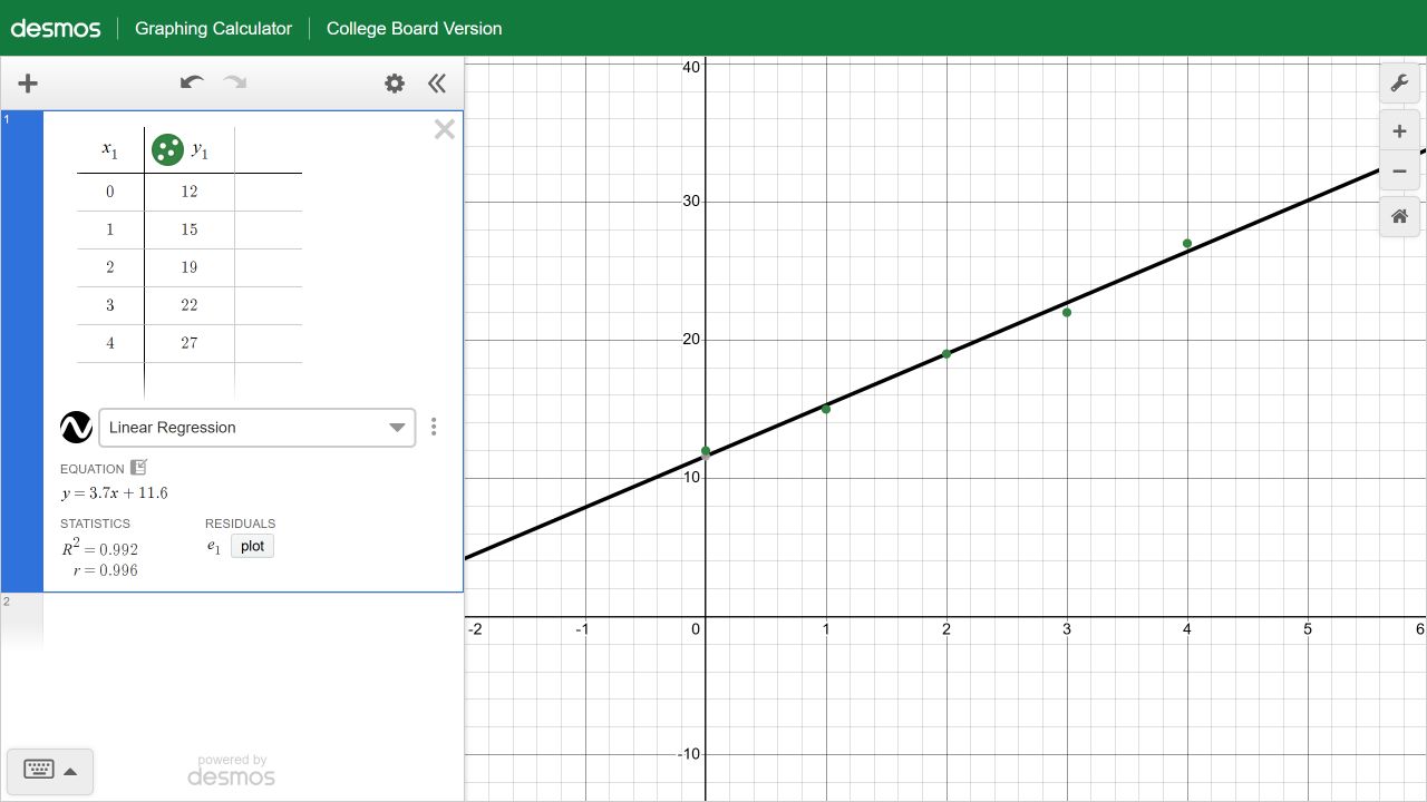
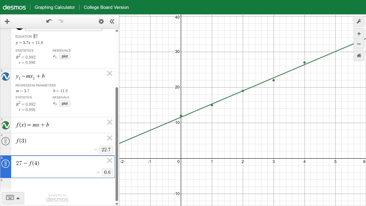
Read m = 3.7 and b = 11.6. Define f(x) = mx + b so later calculations use the fitted parameters, rather than retyping rounded numbers.
Evaluate f(3). The model predicts 22.7; the measured value 22 is a different quantity.
A residual is observed minus predicted. At x = 4, the prediction is 26.4, so enter 27 − f(4).
Predicted y = 22.7. Residual at x = 4 is +0.6: the observation is 0.6 above the fitted line.
Watch for this: A high R² describes fit to these data. It does not establish causation or make every future prediction reliable.
Worked problem
Recover a quadratic and find its maximum
A model gives a ball’s height h, in meters, t seconds after launch. The model is quadratic and matches the table exactly. What is its maximum height, and when does it pass 40 meters on the way down?
Why this approach works
The model type is supplied: height is a quadratic in time. The table therefore creates equations of the form y = ax² + bx + c. Regression finds coefficients satisfying those paired conditions here; with noisy measurements, it would instead find a least-squares approximation.
The vertex formula comes from rewriting ax² + bx + c as a(x + b/(2a))² plus a constant. The square is smallest when its inside is zero, so the turning point is at x = −b/(2a). Because a is negative here, moving away from that point decreases the height.
At an intersection with y = 40, the same time produces height 40 on both graphs. There are two times because the ball passes that height while rising and falling. “On the way down” selects the time after the maximum; the graph does not make that contextual choice for us.
Enter these paired values into a new Desmos table.
x₁
y₁
0	2
1	27
2	42
3	47
Copy the table data
0 2
1 27
2 42
3 47
Paste into an empty expression to create a table. Or choose Add Item → Table and enter the numbers manually.
What to enter
Choose Add Item → Expression. Paste each input into a separate expression line. Use a fresh calculator for each worked problem, including the model comparison. Every example includes its own table and setup.
y_{1}\sim ax_{1}^{2}+bx_{1}+c
h(x)=ax^2+bx+c
-b/(2a)
h(3)
y=40
Do this step by step
Use seconds as the table’s x-values and meters as its y-values. The calculator’s x is the problem’s t.
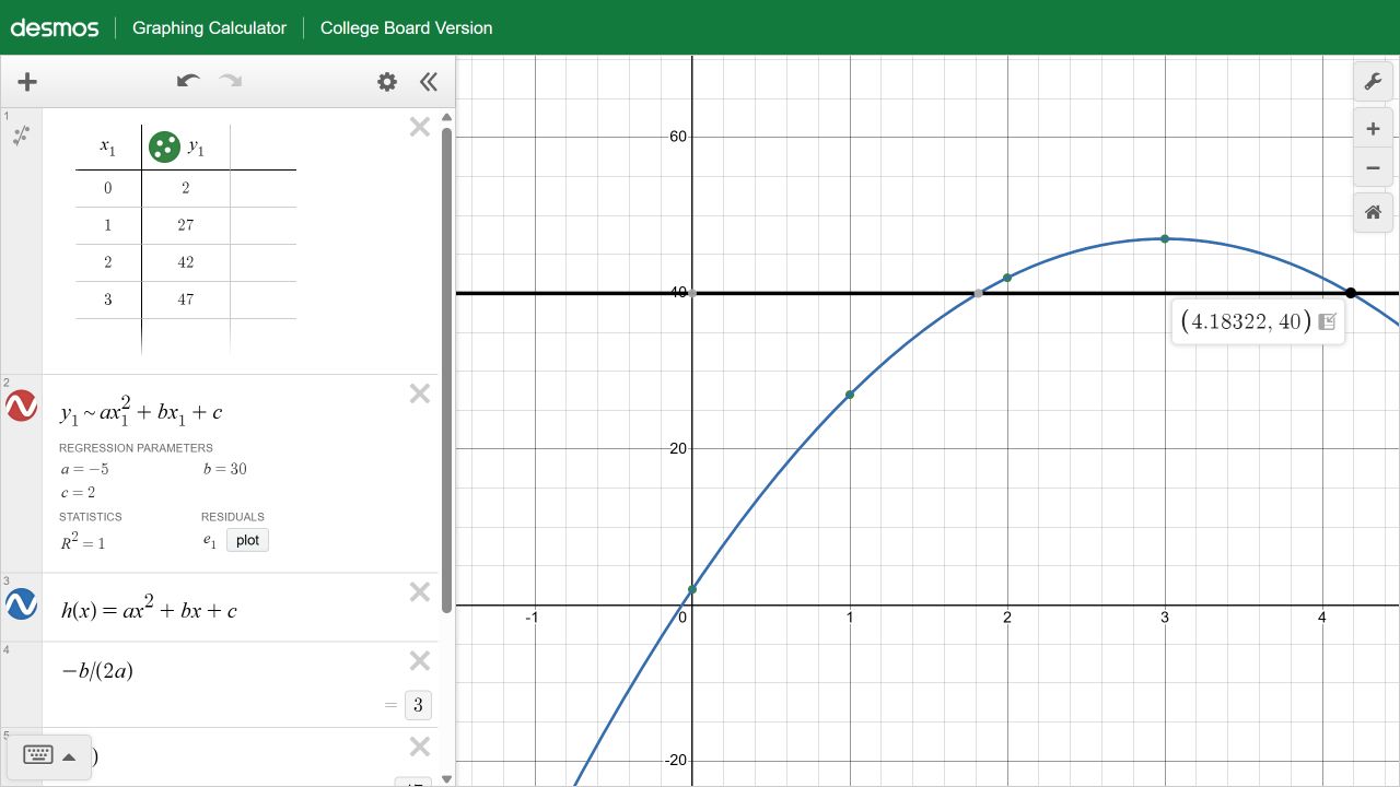
Fit y₁ ~ ax₁² + bx₁ + c. Read a = −5, b = 30, c = 2, so h(t) = −5t² + 30t + 2.
Define h(x), then evaluate −b/(2a). The vertex occurs at t = 3 seconds.
Evaluate h(3) to get the height, 47 meters. Since a is negative, this vertex is a maximum.
Graph y = 40. Select the horizontal line and click its right-hand intersection with the parabola. The calculator shows approximately (4.18322, 40).
Choose the time after the maximum, not the earlier intersection. The relevant x-coordinate is time; the y-coordinate is height.
Maximum height: 47 meters at 3 seconds. On the way down, h = 40 at t = 3 + √(7/5) ≈ 4.18322 seconds.
The fitted coefficients and the later intersection (4.18322, 40) in the SAT calculator. Open full-size screenshot ↗
Check it by hand
Successive height changes are 25, 15 and 5; the second differences are −10. For unit-spaced inputs, 2a = −10, so a = −5.
h(0) = 2 gives c = 2. h(1) = 27 gives −5 + b + 2 = 27, so b = 30.
Complete the square: h(t) = −5(t − 3)² + 47. Its maximum is therefore 47 at t = 3.
Set −5(t − 3)² + 47 = 40. Then (t − 3)² = 7/5, so t = 3 ± √(7/5).
The plus sign gives the time after t = 3. Do not round the displayed 4.18322 to an integer unless the question requests that.
Watch for this: Three data points alone do not prove a relationship is quadratic. Here the question explicitly supplies that model type.
Worked problem
Find a growth rate without losing the time unit
A quantity follows an exponential model exactly. Its values are 500 at year 0, 605 at year 2 and 732.05 at year 4. Find the annual percentage increase. Then use the model to predict the value at year 6 and its doubling time.
Why this approach works
An exponential model represents multiplication by the same factor over equal time intervals. Its form a·bˣ has starting value a at x = 0. Increasing x by 1 multiplies the output by b, so the meaning of b depends on the unit represented by one x-step.
The table uses actual years 0, 2 and 4. A two-year ratio of 1.21 means b² = 1.21, not b = 1.21. Taking the positive square root gives the annual factor 1.1. Subtract 1 to isolate the increase beyond the original 100%, then multiply by 100 to express that increase as a percentage.
For doubling time, divide a·bᵗ = 2a by a to obtain bᵗ = 2. Logarithms bring the unknown exponent down: t·ln(b) = ln(2). Dividing by ln(b) gives the time in the original x-units. Regression estimates a model; this later equation uses that model to answer a different question.
Enter these paired values into a new Desmos table.
x₁
y₁
0	500
2	605
4	732.05
Copy the table data
0 500
2 605
4 732.05
Paste into an empty expression to create a table. Or choose Add Item → Table and enter the numbers manually.
What to enter
Choose Add Item → Expression. Paste each input into a separate expression line. Use a fresh calculator for each worked problem, including the model comparison. Every example includes its own table and setup.
y_{1}\sim ab^{x_{1}}
f(x)=ab^x
100(b-1)
f(6)
\frac{\ln(2)}{\ln(b)}
Do this step by step
Enter actual years 0, 2 and 4. Do not replace them with row numbers 0, 1 and 2.
Fit y₁ ~ ab^(x₁), keeping the entire table variable x₁ in the exponent. The tested paste-ready input above uses explicit braces.
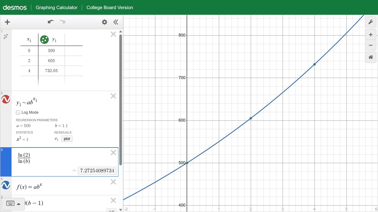
Read a = 500 and b = 1.1. Because x measures years, b is the factor for one year.
Enter 100(b − 1). The result 10 means a 10% annual increase, not 110%.
Define f(x) = abˣ and evaluate f(6). The model gives 885.7805. This is a model projection beyond the observed years.
For doubling time, solve bᵗ = 2 by evaluating ln(2)/ln(b). The calculator gives about 7.27254 years.
Annual increase: 10%. Model prediction at year 6: 885.7805. Doubling time: approximately 7.27254 years.
The SAT calculator returns a = 500, b = 1.1 and a doubling time of about 7.27254 years. Open full-size screenshot ↗
Check it by hand
605 ÷ 500 = 1.21 is the factor across two years.
The positive annual factor satisfies b² = 1.21, so b = 1.1 and the annual increase is 100(1.1 − 1) = 10%.
500(1.1)⁴ = 732.05 checks the third data point. 500(1.1)⁶ = 885.7805.
Doubling means 500(1.1)ᵗ = 1000, or 1.1ᵗ = 2. Taking logs gives t = ln(2)/ln(1.1).
Watch for this: A 21% change across two years is not a 21% annual increase. For noisy data, Log Mode changes what error the fit minimizes; do not switch it simply to obtain a preferred answer. These exact data give the same parameters with it on or off.
Worked problem
Use the structure the question gives you
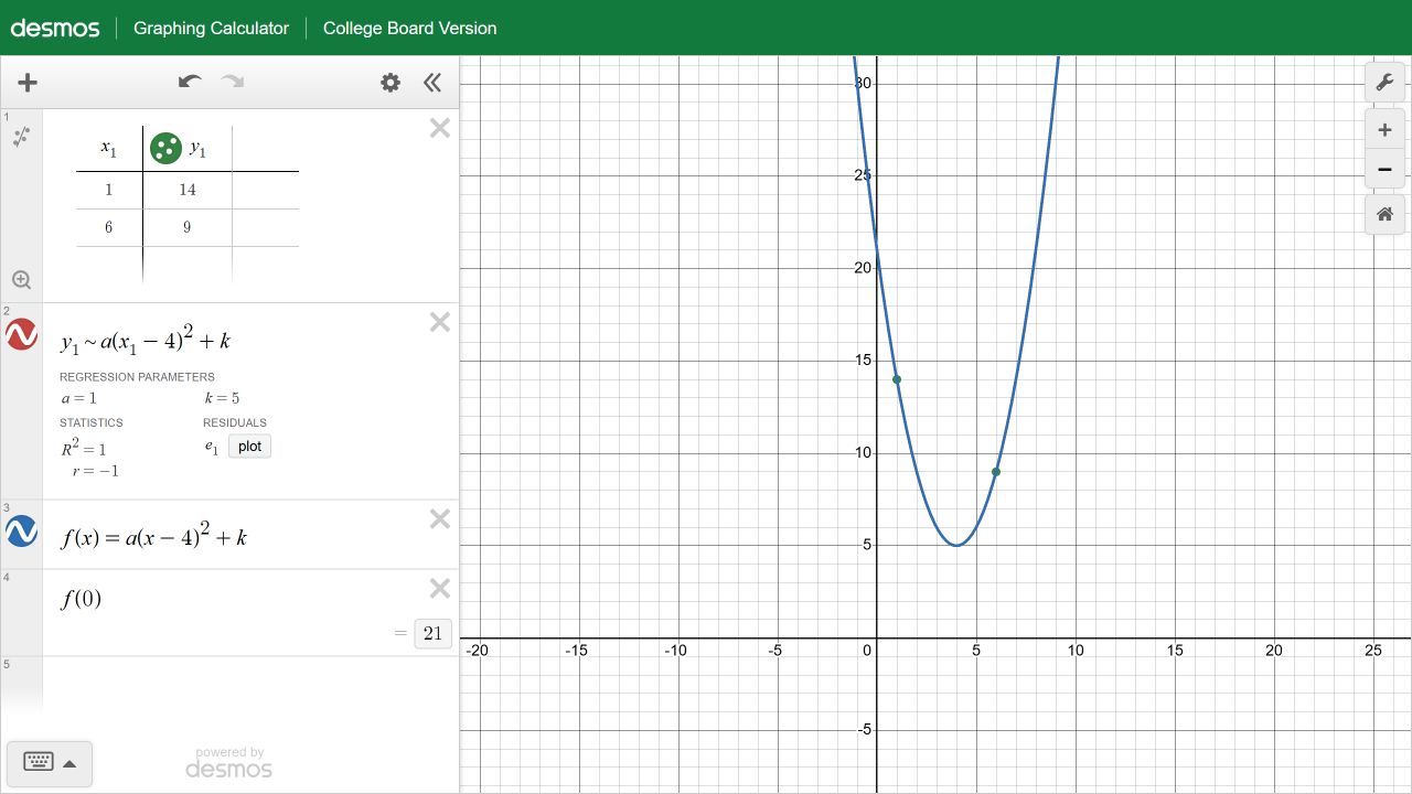
f(x) = a(x − 4)² + k passes through (1, 14) and (6, 9). Find f(0).
Why this approach works
The given form already fixes the vertex’s horizontal coordinate at 4. We must keep that information: fitting a general three-parameter quadratic would throw it away and leave too many unknowns for two points.
At x = 1, the known square (x − 4)² is 9. At x = 6, it is 4. The conditions are therefore 9a + k = 14 and 4a + k = 9. These are two independent equations in a and k, which is why this fit can determine them.
Having two rows is not enough by itself. If both x-values had the same squared distance from 4, the equations could repeat the same information. After finding a and k, evaluating f(0) is just substitution into the specific function they determine.
Enter these paired values into a new Desmos table.
x₁
y₁
1	14
6	9
Copy the table data
1 14
6 9
Paste into an empty expression to create a table. Or choose Add Item → Table and enter the numbers manually.
What to enter
Choose Add Item → Expression. Paste each input into a separate expression line. Use a fresh calculator for each worked problem, including the model comparison. Every example includes its own table and setup.
y_{1}\sim a(x_{1}-4)^2+k
f(x)=a(x-4)^2+k
f(0)
Do this step by step
Notice that the question already gives the horizontal coordinate of the vertex: 4. Only a and k are unknown.
Enter the two points in the table. Use the supplied form in the regression instead of fitting an unrestricted ax² + bx + c.
Read a = 1 and k = 5. Define f(x) = a(x − 4)² + k.
Evaluate f(0). The calculator returns 21.
If Zoom Fit hides the vertex, zoom out or adjust the axes. Fitting the data points to the window does not guarantee that every important feature is visible.
f(0) = 21. The function is f(x) = (x − 4)² + 5, with minimum 5 at x = 4.
Subtract to get 5 = 5a, hence a = 1. Then k = 9 − 4 = 5.
Finally f(0) = (0 − 4)² + 5 = 16 + 5 = 21.
Watch for this: Two points do not determine a general quadratic with three unknown coefficients. They determine this function because the supplied structure reduces the unknowns to two.
Worked problem
A perfect fit can still be the wrong model
A quantity follows an exponential model exactly: 500 at year 0, 605 at year 2 and 732.05 at year 4. Can a quadratic also fit all three points? Does R² = 1 tell you which model should be used for year 6?
Why this approach works
R² summarizes how closely a chosen model matches the observed y-values. It does not identify the physical rule that generated them. Three distinct x-values can determine a quadratic, so an exact quadratic fit through three points is not surprising.
Both candidate functions satisfy every condition in the small table. They are still different functions: their formulas do not have to agree at x = 6, which was not in the table. That is why we explicitly compare predictions outside the observed inputs.
The phrase “exponential model” supplies information beyond the points. Respecting that condition selects the exponential prediction. Choosing whichever model has a perfect displayed statistic would ignore part of the question.
Enter these paired values into a new Desmos table.
x₁
y₁
0	500
2	605
4	732.05
Copy the table data
0 500
2 605
4 732.05
Paste into an empty expression to create a table. Or choose Add Item → Table and enter the numbers manually.
What to enter
Choose Add Item → Expression. Paste each input into a separate expression line. Use a fresh calculator for each worked problem, including the model comparison. Every example includes its own table and setup.
y_{1}\sim ab^{x_{1}}
f(x)=ab^x
f(6)
y_{1}\sim px_{1}^{2}+qx_{1}+r
g(x)=px^2+qx+r
g(6)
f(6)-g(6)
Do this step by step
Open a fresh calculator and enter the table shown here. Fit y₁ ~ ab^(x₁): a = 500 and b = 1.1. Define f(x) = abˣ and evaluate f(6) = 885.7805 before adding the quadratic. Use new parameter letters p, q and r so this experiment does not overwrite a and b.
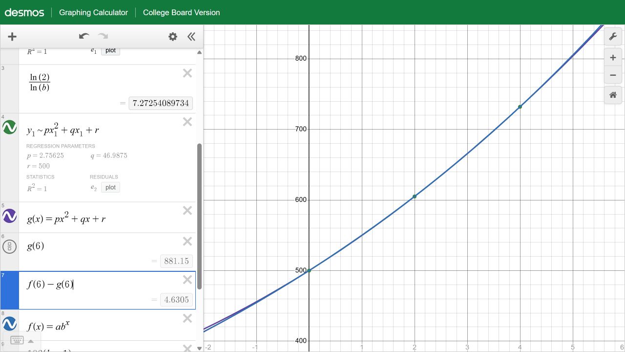
Fit the same table to y₁ ~ px₁² + qx₁ + r. The calculator gives p = 2.75625, q = 46.9875 and r = 500.
Define g(x) from those parameters. Both models match all three observed points and show R² = 1.
Evaluate g(6): 881.15. Compare it with f(6) = 885.7805. The predictions differ by 4.6305.
Choose the model supported by the question’s stated relationship. A perfect fit to three points does not prove that relationship continues between or beyond them.
Both fit the three points, but their year-6 predictions differ. If the problem states exponential growth, use 885.7805 from the exponential model.
The quadratic also shows R² = 1, yet g(6) = 881.15 differs from the exponential prediction. Open full-size screenshot ↗
Check it by hand
The quadratic’s constant term is 500 because x = 0 gives y = 500.
At x = 2: 4p + 2q = 105. At x = 4: 16p + 4q = 232.05.
Subtract twice the first equation from the second: 8p = 22.05, so p = 2.75625. Then q = (105 − 4 × 2.75625)/2 = 93.975/2 = 46.9875.
g(6) = 2.75625(36) + 46.9875(6) + 500 = 881.15.
885.7805 − 881.15 = 4.6305.
Watch for this: Do not choose a higher-degree model solely because its R² is larger. A displayed 1 can also reflect rounding; check the model, residuals and context.
Try the hard SAT toolkit next
Work through systems, one-solution parameters, radicals, rational equations, transformations, inequalities and domain traps. Then try three guided problems yourself.
A graph can suggest roots, a maximum, or a parameter value. Check exact values with algebra, keep excluded inputs, and make sure the window has not hidden another solution. Keep intermediate precision and round only as requested.
Sources and calculator notes
Desmos documents regression models, residuals, the effect of Log Mode and numerical fitting limitations. Its testing calculators can differ from the general calculator. College Board includes nonlinear equations, functions and systems in SAT Advanced Math. The examples and algebra here were independently worked for this lesson.